How to Perform a Student’s T-Test in SAS [Examples]

In this article, we discuss how to perform a Student’s t-test in SAS.

The Student’s t-test is a method of testing hypotheses about the mean of one or two groups. With a t-test, one can determine whether the means of two groups are statically different, or whether the mean of one group is different from a known value.

In SAS, the easiest way to perform a Student’s t-test is by using the TTEST procedure (PROC TTEST). With this procedure, one can perform a one-sample t-test, two-sample t-test, or a paired t-test. Given the input parameters, the TTEST procedure calculates the test statistics, the corresponding p-value, and confidence intervals.

In this article, we first discuss briefly which types of t-tests exist and how to select the correct one. Next, we will show how to use PROC TTEST to perform each type of t-test and how to interpret the results. We support all our explanations with examples and SAS code that you can use directly in your own projects.

Types of Student’s T-Tests

As mentioned before, the TTEST procedure can perform different types of t-test (one-sample, two-sample, or paired t-test), but how do you select the right one?

The diagram below helps you choose the right t-test for your situation.

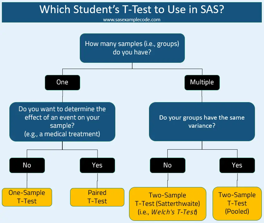
To summarize, you use the:

• One-sample t-test when you have one sample (i.e. group) and you want to determine if its mean is stastically different from 0 or any other known value.
• Paired t-test when you have one group and want to measure the effect of some event. For example, a medical treatment.
• Two-sample t-test (Satterthwaite method or Welch’s t-test) when you want to compare two groups with different variances.
• Two-sample t-test (Pooled method) when you want to compare two groups with the same variance.

Perform a Student’s T-Test

The TTEST procedure in SAS performs t-tests of different types and computes confidence intervals. It also generates some plots (e.g., QQ-plots) that facilitate analyzing the results.

Irrespectively of the type of t-test, one always needs to complete at least the following steps to perform a t-test in SAS:

1. Start the procedure with the PROC TTEST statement.
2. Define the input dataset with the DATA=-option.
3. Specify the variable that needs to be tested with the VAR statement.
4. Run the procedure with the RUN statement.

Next, we will discuss how to modify these steps to perform each type of the Student’s t-test.

Perform a One Sample T-Test

The most basic t-test is the one-sample t-test which checks whether the mean of a sample is significantly different from zero or another known value.

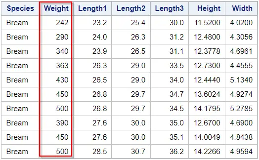
In the examples below, we will analyze the weight of breams (of species of fish).

Test the Sample Mean Against Zero

The image below shows the default hypothesis of a one-sample t-test. In other words, it checks whether the sample mean (µ) is significantly different from zero.

To check in SAS whether the mean of a sample is significantly different from zero, you only need to provide the name of the input dataset and the variable you want to test. You do this with the DATA=-option and the VAR statement.

Additionally, you can use the ALPHA=-option to specify the confidence level. For example, you can use ALPHA=0.01 for a 99% confidence level. By default, SAS performs the t-test with a confidence level of 95%.

In the example below, we use the TTEST procedure to determine if the mean weight of the Bream species differs from 0. To select only the Bream species, we use the WHERE=-option to filter the input data.

proc ttest data=sashelp.fish (where=(Species = "Bream"))
    alpha=0.05;
    var weight;
run;

The image below shows the report that PROC TTEST generates.

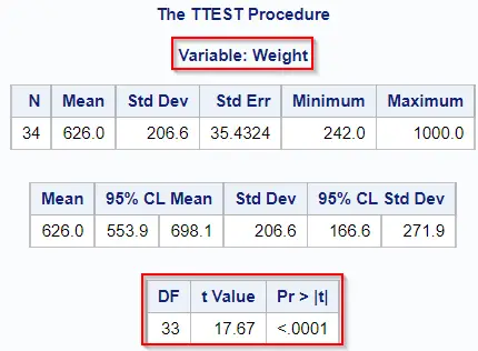
Highlighted in red, we see the degrees of freedom (DF = 33), the value of the test statistic (t Value = 17.67), and the p-value. Since the p-value is lower than our confidence level of 0.05, we reject the null hypothesis and conclude that the mean weight of the bream species is significantly different from zero.

Test the Sample Mean Against Another Known Value

Alternatively, we could specify a more realistic null hypothesis for the mean weight of a fish, e.g. 600 grams.

To specify the null hypothesis of a one-sample t-test in SAS, you can use the H0=-option. With this option, you can define the known value against which SAS tests the sample mean.

In the example below, we use the H0=-option to test whether the mean weight is equal to 600 grams.

proc ttest data=sashelp.fish (where=(Species = "Bream"))
    alpha=0.05
    H0=600;
    var weight;
run;

The image below shows the results of our new hypothesis. (Unfortunately, SAS doesn’t add the null hypothesis to the report).

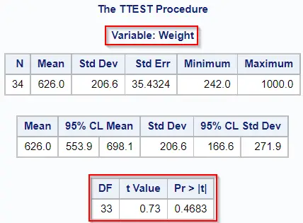
Because the p-value (0.4683) is higher than our confidence level of 0.05, we don’t reject the null hypothesis and conclude that the mean weight is not statistically different from 600 grams.

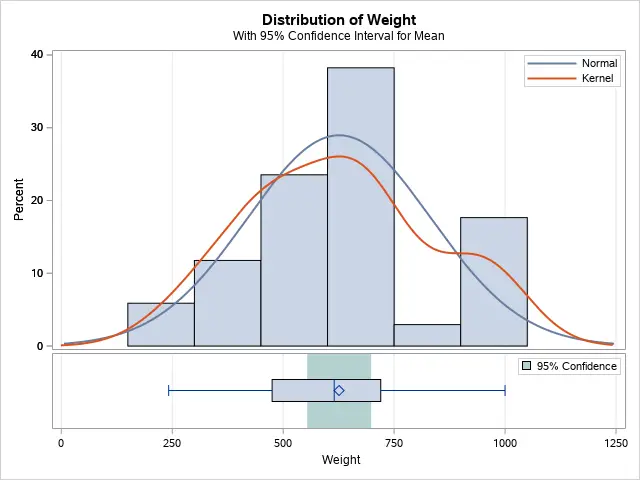
Besides the degrees of freedom, the value of the test statistic, and the p-value, the report also contains the confidence intervals for the mean and the standard deviation. Additionally, the PROC TTEST procedure creates some extra plots to facilitate your analysis.

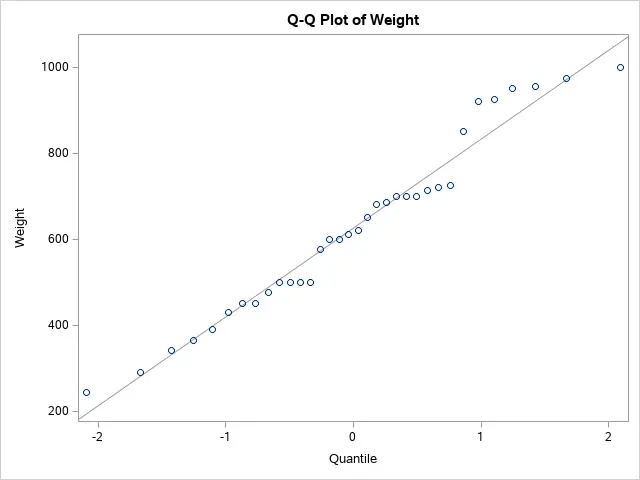
One of the main assumptions of the t-test is that your data (e.g., the weight of fish) follows a normal distribution. To check this assumption, you can use the Q-Q plot. If all data points are close to the main diagonal, then it follows a normal distribution and, therefore, meets the assumption.

For example, the Q-Q plot below confirms that the weight of bream fish is normally distributed.

Perform a Two Sample T-Test

The second type of t-test is the two-sample t-test, also known as the independent samples t-test.

The two-sample t-test is a method to check if the sample means (µ₁ and µ₂) of two independent samples (i.e., different groups) are equal. The alternative hypothesis (H₁) assumes that the means are different. See the image below.

Instead, if you want to check the means of two variables from the same group, you need the paired t-test.

To perform a two-sample t-test in SAS, you use the TTEST procedure in combination with the CLASS statement. These are the steps:

1. Start the TTEST procedure with the PROC TTEST statement.
2. Define the input dataset with the DATA=-option.
3. Specify the variable that defines the two groups/samples with the CLASS statement.
4. Define the variable you want to test with the VAR statement.
5. Execute the TTEST procedure with the RUN statement.

A prerequisite to performing the two-sample t-test is that the input dataset is ordered by the variable that defines the groups (i.e., the variable of the CLASS statement). One way you can order a dataset is with the SORT procedure.

Besides an ordered dataset, SAS also requires that the data contains exactly two groups. If your data doesn’t meet this requirement, then two errors can occur:

1. ERROR: The CLASS variable does not have two levels. In this case, you might want to perform a one-sample t-test.

2. ERROR: The CLASS variable has more than two levels. In this case, you might want to perform the ANOVA test which determines if (more than two) groups are statistically different. Alternatively, you can change the CLASS statement for the BY statement, and do a one-sample t-test for all groups independently.

In the example below, we use the TTEST procedure to compare the average weight of two fish species. We use a confidence level of 95% (ALPHA=0.05).

proc sort data=sashelp.fish
    out=work.fish (where=(Species in ("Bream" "Parkki"))
	keep=Species Weight);
    by Species;
run;
 
proc ttest data=work.fish
    alpha=0.05;
    class Species;
    var weight;
run;

How to Interpret the Results of a Two-Sample T-Test

The next image shows the output of a two-sample t-test in SAS.

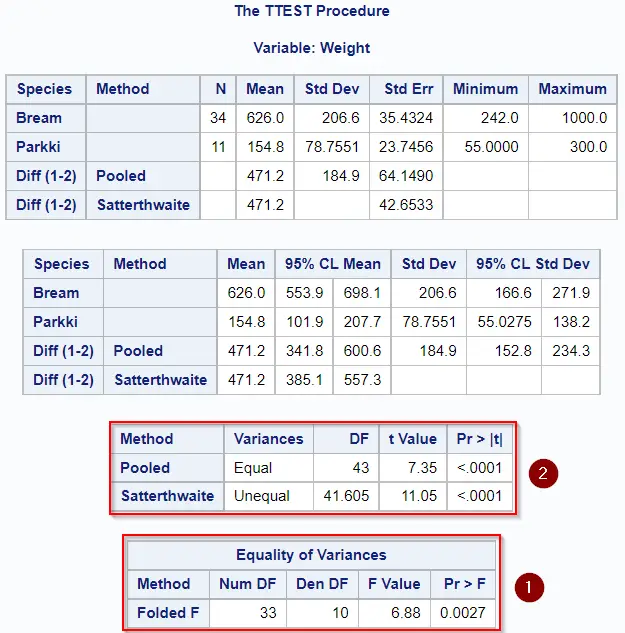
In order to draw the correct conclusion and (not) reject the null hypothesis, you need to follow the next steps:

1. Check the results of the Equality of Variances test.
2. Select the correct method to draw a conclusion.

If the p-value of the Equality of Variances test is greater than your significance level (e.g., 0.05), then we assume that the variances are equal and you should use Pooled method to draw the correct conclusion. Otherwise, the Satterthwaite method (i.e., the Welch’s t-test) is the one you need.

So, in our example, the p-value of the Equality of Variance test is lower than 0.05, and hence significant. Therefore, we should use the Satterthwaite method to draw conclusions about the two-sample t-test. Since the p-value of the Satterthwaite is also lower than 0.05, we reject the null hypothesis and conclude that the means of the two groups are statistically different.

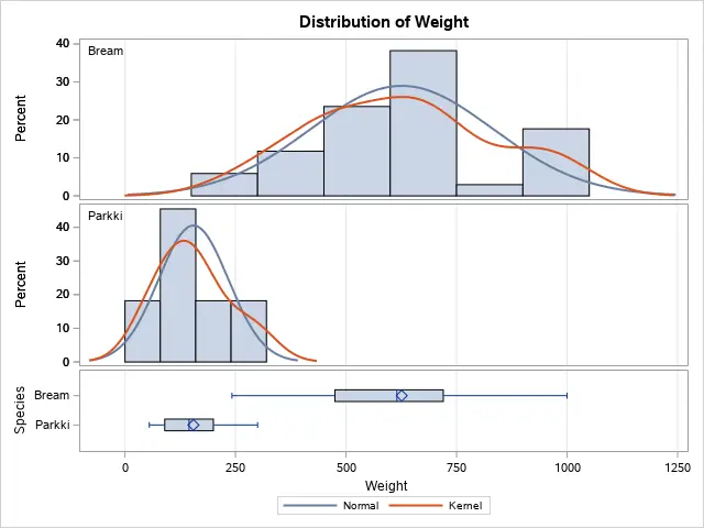
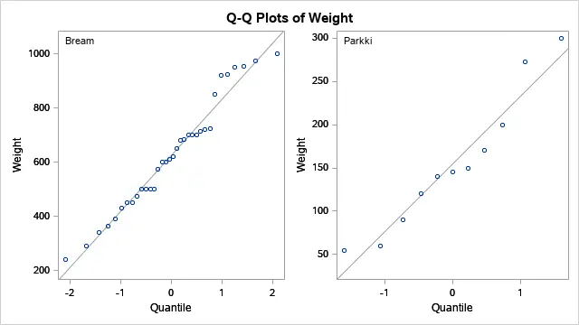
Besides the test statistics, p-values, and confidence intervals, the TTEST procedure also generates two plots. These plots might help you to support your conclusion (the histogram) or test the normality assumption (the Q-Q plot).

Perform a Paired T-Test

The third type of t-test is the paired t-test.

In contrast to the two-sample t-test, the paired t-test determines whether the means of two variables of the same group are equal. This type of test is frequently used to compare the means before and after a certain event. For example, a medical treatment.

Instead, if you want to test the means of the same variable from different groups, you need the two-sample t-test.

To perform a paired t-test in SAS, you need to follow these steps:

1. Start the TTEST procedure with the PROC TTEST statement.
2. Define the input data with the DATA=-option.
3. Specify the two variables with the PAIRED statement. (You must separate the two variables with in asterisk (*)).
4. Run the TTEST procedure with the RUN statement.

Note that you can’t use the CLASS statement in a paired t-test. If you want to test multiple groups, you either need the BY statement or the ANOVA test.

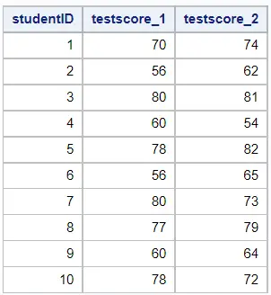
In the example below, we create a dataset of 10 students. Each student has taken two exams; one before taking a certain course, and one after taking the course. We want to know if taking the course has a significant (positive) effect on the test scores.

data work.test_scores;
    infile datalines dlm=",";
    input studentID testscore_1 testscore_2;
    datalines;
1, 70, 74
2, 56, 62
3, 80, 81
4, 60, 54
5, 78, 82
6, 56, 65
7, 80, 73
8, 77, 79
9, 60, 64
10, 78, 72
;
run;
 
proc ttest data=work.test_scores;
    paired testscore_2 * testscore_1;
run;

The images below show the output of the TTEST procedure of the paired t-test.

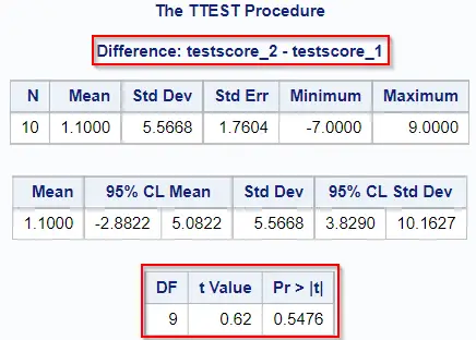
Based on the p-value of 0.5476, we don’t reject the null hypothesis and therefore conclude that taking the course hasn’t had a (positive) effect on the test scores.

The following plots show the differences between the test score from various perspectives and might help you to support your conclusion.

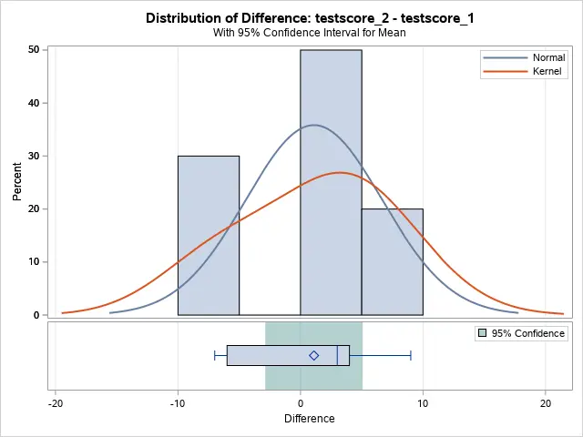
The image above shows clearly why we didn’t reject the null hypothesis, namely a zero difference lies within the 95% confidence interval.

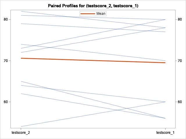
The next plot also shows that the test scores on average haven’t changed much.

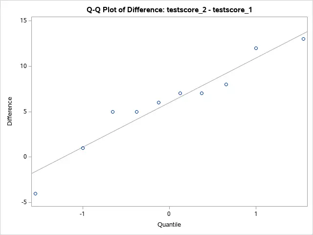
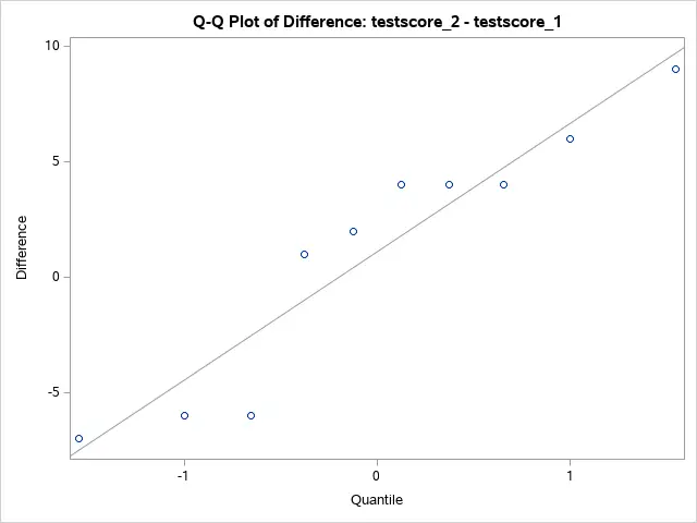
One of the main assumptions of the paired t-test is that the differences are normally distributed. We can check this assumption with the Q-Q plot. If the differences are on or near the main horizontal line, then we conclude that the differences follow a normal distribution.

The next example shows a situation where the test scores before and after taking the course are significantly different.

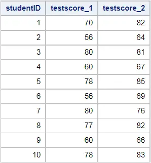
data work.test_scores2;
    infile datalines dlm=",";
    input studentID testscore_1 testscore_2;
    datalines;
1, 70, 82
2, 56, 64
3, 80, 81
4, 60, 67
5, 78, 85
6, 56, 69
7, 80, 76
8, 77, 82
9, 60, 66
10, 78, 83
;
run;
 
proc ttest data=work.test_scores2;
    paired testscore_2 * testscore_1;
run;

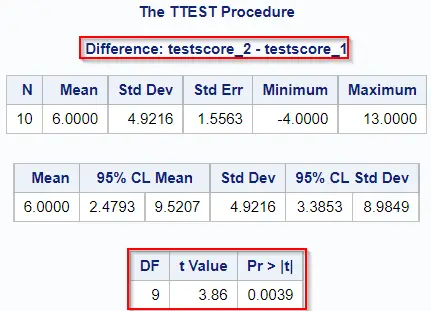
In this example, we do reject the null hypothesis of the paired t-test and conclude that taking the course has had a (positive) effect on the test scores.

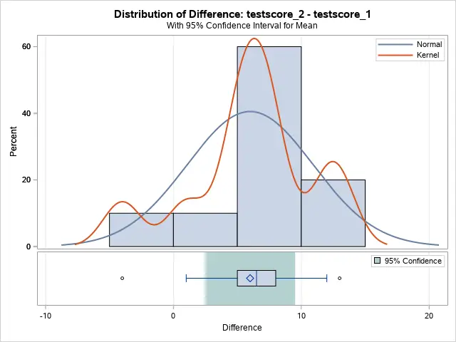
The plot of the Distribution of Difference (see below) supports this conclusion as the zero difference doesn’t lie within the 95% confidence interval.

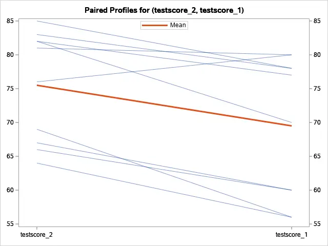
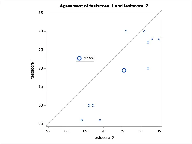
The Paired Profiles and Agreement plots also demonstrate that there is a clear difference between the two test scores.

The Q-Q plot confirms that the differences follow a normal distribution. Therefore, one of the main assumptions holds and we can trust our conclusion about rejecting the null hypothesis.