In this article, we explain how to run a simple linear regression in SAS. That meas, we try to model the linear relationship between one dependent variable and one independent variable.
In short, you run a simple linear regression in SAS with the PROC REG procedure. This procedure models the relationship between two numeric variables and returns a report of the results (parameter estimates, goodness-of-fit statistics, etc.).
Although PROC REG is the preferred method of most SAS users, there exist many other ways to run a simple linear regression. Therefore, we discuss 3 of them, namely:
- PROC REG (writing SAS code)
- PROC GLM (writing SAS code)
- SAS Studio (point-and-click interface)
We will discuss the basics of these methods (i.e., the syntax, the results, and the output). Also, we provide examples where we model the relationship between the variables weight (dependent variable) and height (independent variable) from the CLASS dataset in the SASHELP library.
Contents
How to Run a Simple Linear Regression with PROC REG
The first method to run a simple linear regression is with the PROC REG procedure, a general-purpose procedure for regression in SAS. This method is straightforward to program and returns a report with the most important statistics and parameters.
These are the steps to run a simple linear regression in SAS with PROC REG:
- Start the PROC REG procedure
You start the procedure with the PROC REG statement.
- Specify the input dataset
You specify the name of the input dataset with the DATA=option. You can use either a dataset from the work library or a permanent library.
- Define the relationship between your variables
You define the relationship between your variables with the MODEL statement. The statement starts with the MODEL keyword, followed by the dependent variable, an equal sign, and the independent variable.
- Finish and execute the PROC REG procedure
You use the RUN statement to finish and execute your code.
The code below provides an example of how to use PROC REG to run a simple linear regression in SAS.
proc reg data=sashelp.class;
    model weight=height;
run;
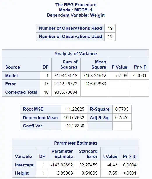
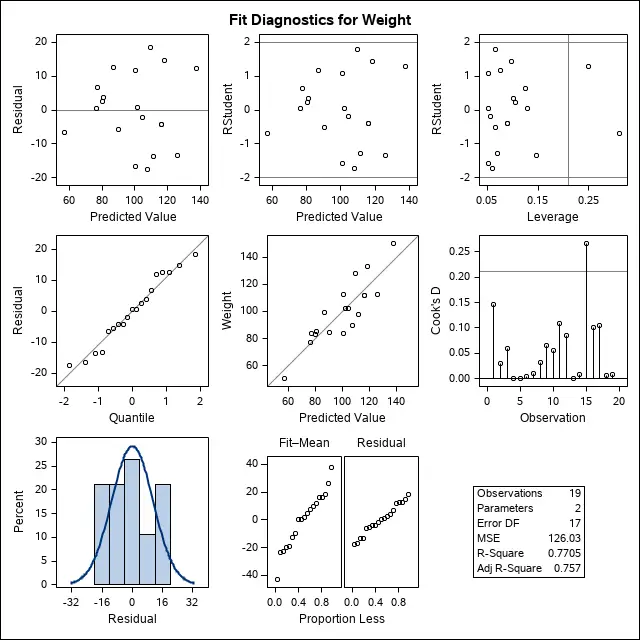
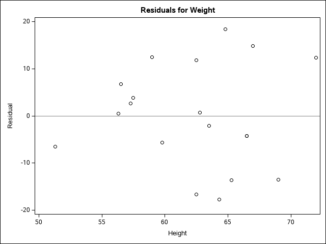
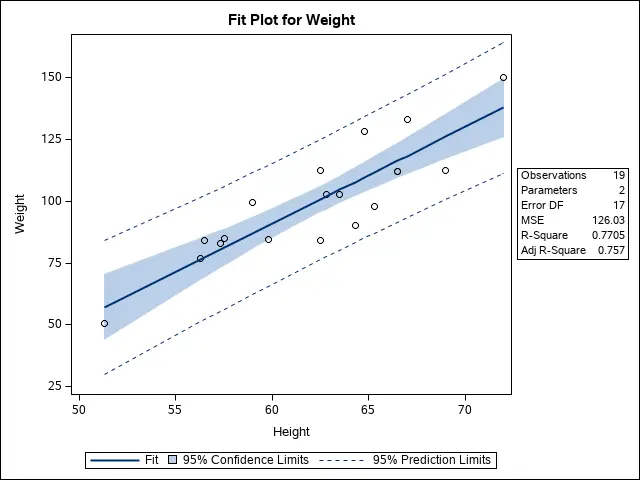
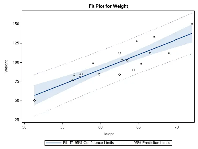
When you use PROC REG to create a linear model, SAS creates a report that contains the analysis of variance, parameter estimates, and several scatterplots and histograms.
How to Create an Output Table with Parameter Estimates in PROC REG
By default, PROC REG generates a report with the parameter estimates for the intercept and slope of the regression. However, it doesn’t save these estimates in a dataset for later use.
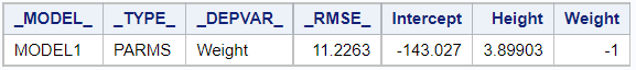
However, you can add the OUTEST=-option to the PROC REG statement to create a SAS dataset with the parameter estimates. Besides the estimates for the intercept and slope, the output dataset also contains the Root Mean Squared Error (RMSE) statistic.
As an example, we use the OUTEST=-option to create the dataset param_estimates with the parameter estimates of the PROC REG procedure.
proc reg data=sashelp.class
    outest=work.param_estimates;
    model weight=height;
run;
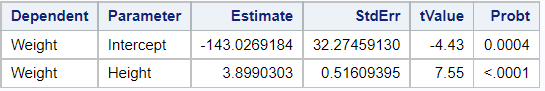
The image below shows that the estimates for the intercept and slope are -143.0 and 3.8, respectively.
How to Run a Simple Linear Regression with PROC GLM
The second method to run a linear regression in SAS is with the PROC GLM procedure.
The PROC GLM procedure is very similar to the PROC REG procedure. In fact, the code to create a simple linear model is identical. The only difference between the two procedures is the report SAS generates.
You create a simple linear regression with the PROC GLM statement and the MODEL statement. First, you use the PROC GLM statement to define the input and, optionally, the output dataset. Then, with the MODEL statement, you specify the relationship between the dependent and independent variables.
This is the SAS code to run a simple linear regression with PROC GLM.
proc glm data=sashelp.class;
    model weight=height;
run;
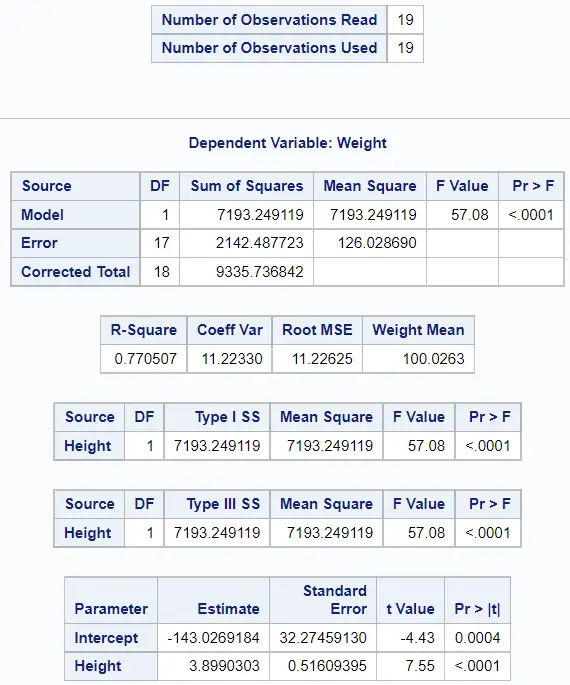
The images below show the default report.
By default, PROC GLM only generates a report. That means that SAS doesn’t save the parameter estimates for the intercept and slope in a separate table. However, you can use the ODS OUTPUT statement and the ParameterEstimates keyword to create a table with the parameter estimates.
ods output ParameterEstimates = <table-name>;
The code below shows how to use the ODS OUTPUT statement.
ods output ParameterEstimates = work.param_estimates;
proc glm data=sashelp.class;
    model weight=height;
run;
As you can see, the PROC REG and PROC GLM seem similar, but there are some differences. These are the main difference between the default behaviour of PROC REG and PROC GLM:
| PROC REG | PROC GLM | |
|---|---|---|
| Intended use | Linear Regression Models | Generalized Linear Models |
| Analysis of Variance (Report) | Yes | Yes |
| Parameter Estimates (Report) | Yes | Yes |
| Fit Plot | Yes | Yes |
| Type 1 / 3 Sum of Squares | No | Yes |
| Fit Diagnostics Plot | Yes | No |
| Parameter Estimates (Output Table) | With OUTEST=-option | With ODS OUTPUT statement |
How to Run a Simple Linear Regression with SAS Studio
If you don’t want to write code to run a simple linear regression, then you can use SAS Studio instead. SAS Studio provides a point-and-click interface that guides you through the process of creating a simple linear regression model So, no coding is required.
These are the steps to run a simple linear regression with SAS Studio.
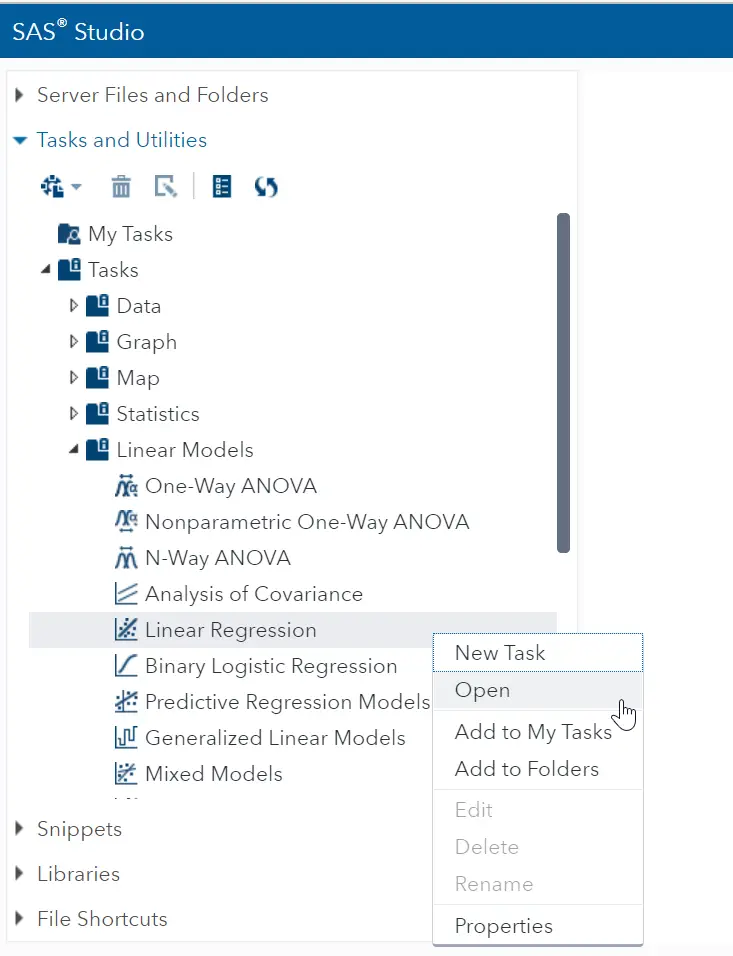
1. Open the Linear Regression Task
In order to run a simple linear regression in SAS Studio, you use the “Linear Regression” task. You find this task in the “Tasks and Utilities” pane under Tasks > Linear Models. Right-click the Linear Regression task and select Open to begin creating a linear regression.
2. Select the Input Dataset
Once you’ve opened the Linear Regression task, you can start building a Simple Linear Regression. The first step is to select the input dataset.
You can select the input dataset in the Data tab under the Data option. You can either write the name of your dataset or browse for it by clicking the table icon. After selecting the input dataset, you could add filters to the data.
In the example below we select the CLASS dataset from the SASHELP library.

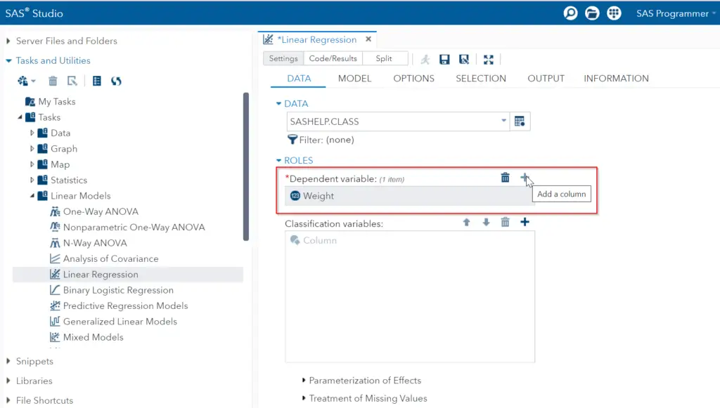
3. Select the Dependent Variable
When you’ve selected the input dataset, you can define the Roles of your regression model. That is to say, the dependent and independent variables. First, you need to select the dependent variable.
You select the dependent variable by clicking on the plus icon. A new window will show you a list of all numeric variables in your dataset. Select one variable and click the OK button to assign this variable the role of the dependent variable.
4. Select the Independent Variable (Part 1)
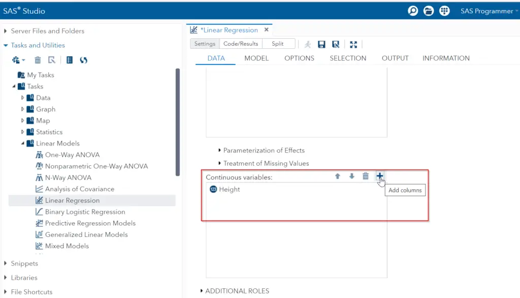
Once you have defined the dependent variable, you need to select the independent variable. This is a two-step process. First, you need to select the numeric variables that enter the model (except the dependent variable).
To select the numeric variables, scroll down in the Data tab until you find the Continuous Variables section. By clicking on the plus icon, a new window pops up with all the numeric variables in the dataset. Select a variable and click the OK button to use this variable in the model.
Note that you could select more than one variable. However, since we a running a simple linear regression model, we only select one variable.
5. Select the Independent Variable (Part 2)
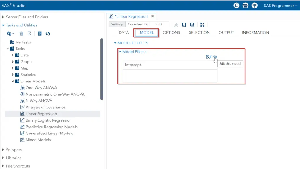
After you have selected all numeric variables that enter the model, you can define the independent variable.
To select the independent variable of your simple linear regression model, go to the Model tab. By default, all linear regression models have an intercept. To add an independent variable click the Edit button. A new window pops ups.
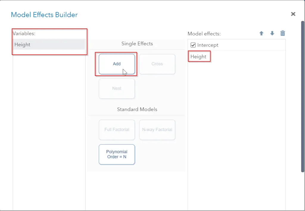
In this window, select the name of the variable and click the Add button. By doing so, the variable will show up in the list of Model effects on the right. Scroll down and click the OK button to close this window.
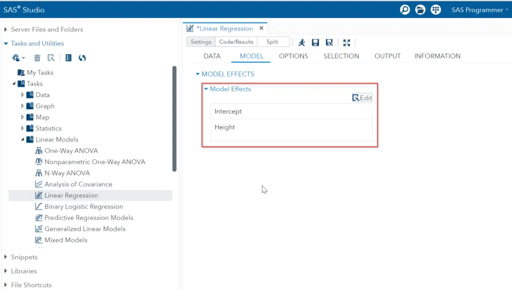
Now, the variable will appear in the list of Model Effects under the intercept
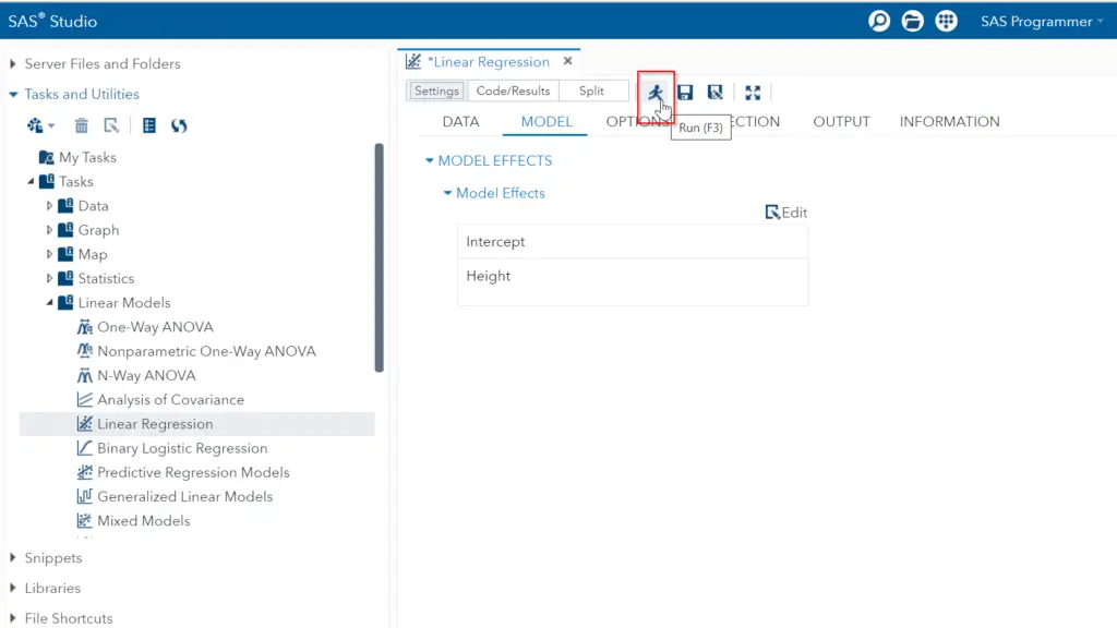
6. Run the Simple Linear Regression
Now that you’ve selected the dependent and independent variables, you can run your model. You do so by click on the RUN button o pressing F3.
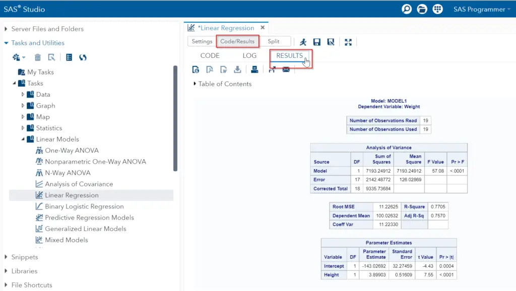
7. Check the Results
You can check the results of the linear regression model by clicking on the Code/Results section and selecting the Results tab.
The Results tab shows a number of tables and graphs with the results of the regression model. You can use these tables and graphs to find the parameters of the model and to check if all assumptions of a linear model hold.
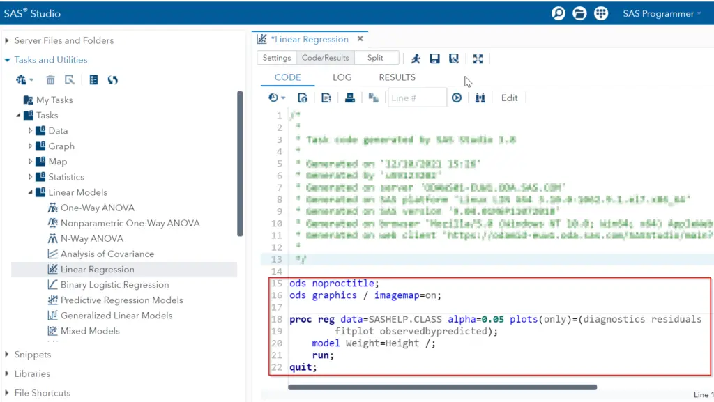
8. Examine the SAS Code (Optionally)
As the steps above show, you don’t need to write one line of code to run this simple linear regression. However, if you are interested in the SAS code, you can check the Code tab. Here you will find the code SAS has created automatically.
As the images above demonstrate, you don’t need to write code to run a simple linear regression in SAS Studio. Moreover, SAS Studio offers a lot of extra options. However, SAS Studio doesn’t offer the option to create an output dataset with the parameter estimates for the intercept and slope. If you absolutely need the parameter estimates in a dataset, you could copy the code from SAS Studio and add the OUTEST=-option to your code.
This video shows how to run a simple linear regression in SAS Studio.