Visualizing data in a scatter plot helps to understand data, highlight trends, and detect outliers. Therefore, in this article, we discuss how to create a scatter plot in SAS.
The easiest way to create scatter plots in SAS is with the SGPLOT procedure. You only need to specify the names of the input dataset, the x-variable, and the y variable and SAS will generate a neat scatter plot.
You can enhance your scatter plot by adding extra options or statements to your code. For example, to create a grouped scatter plot or add regression lines.
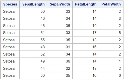
In this article, we show how to create a basic scatter plot, as well as to most common options SAS offers to modify the plot. All examples are based on the famous Iris flower dataset that is available in the SASHELP library. We will use the columns SepalLength and PetalLength to make the scatter plots.
Contents
How to Create a Basic Scatter Plot in SAS
Although there are different ways to create a scatter plot in SAS, the easiest and most intuitive way is with PROC SGPLOT.
The SGPLOT procedure creates one or more plots (e.g., a scatter plot and a regression plot) and overlays them on a single set of axes. The procedure allows you to create different types of plots (e.g. boxplots, bar charts, histograms, etc.) and to control their appearance with extra options and statements.
These are the steps to create a scatter plot in SAS:
- Start the SGPLOT procedure
You start the SGPLOT procedure with the PROC SGPLOT keywords.
- Specify the input dataset
You define the name of the input data with the data=-option. This option starts with the data keyword, followed by an equal sign and the name of your dataset.
- Create the scatter plot
You create the actual scatter plot with the SCATTER statement. This statement starts with the scatter keyword, followed by the variable for the x-axis, and the variable for the y-axis.
You can add additional options to, for example, create a grouped scatter plot. - Optionally, add statements to enhance the scatter plot
You can add extra statements to the SGPLOT procedure to enhance the scatter plot. For example, you can add a legend, a regression line, or a title.
- Finish and run the SGPLOT procedure
You finish and execute the code of the SGPLOT procedure with the RUN statement.
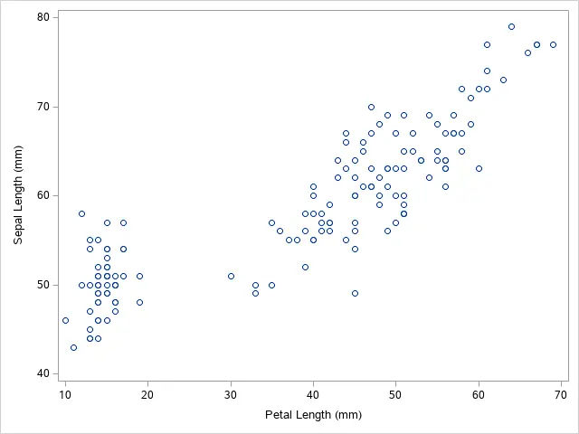
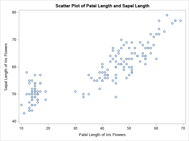
The SAS code in the example below generates a basic scatter plot and shows the relationship between the variables SepalLength and PetalLength.
proc sgplot data=sashelp.iris;
    scatter x = petallength  y = sepallength;
run;
It seems that there exists a positive correlation between the SepalLength and the PetalLength of the Iris flowers.
How to Create a Scatter Plot with Groups
A basic scatter plot gives you a first insight into the distribution of your data. However, if your data can be split into different groups, then a grouped scatter plot might be more useful.
You create a grouped scatter plot in SAS with the group=-option. The option starts with the group keyword, followed by an equal sign and the name of the variable that defines the groups. This option is an additional argument of the scatter statement and must therefore be placed after a forward slash at the end of the statement.
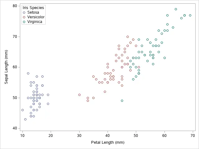
The example below shows how to create one scatter plot where each species is differentiated using a distinctive color.
proc sgplot data=sashelp.iris;
    scatter x = petallength  y = sepallength / group=species;
run;
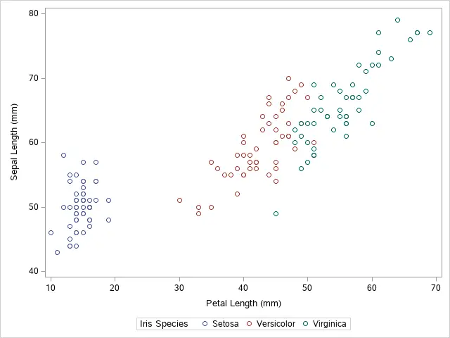
By default, SAS displays the groups in a grouped scatter plot with circles of different colors (e.g., blue, red, and green).
You can change the appearance (type of marker and color) of each group in a scatter plot with the styleattrs statement and the datasymbols=-option. The datasymbols=-option defines the symbol/marker of each group.
SAS offers an extensive list of different symbols, such as circles, asterisks, arrows, etc. Here, you can find a complete list of symbols.
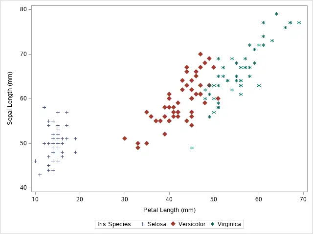
In the example below, we show how to control the symbol of each group in the scatter plot. We use the plus, diamond, and asterisk symbols.
ods graphics / attrpriority=none;
proc sgplot data=sashelp.iris;
    styleattrs datasymbols=(Plus DiamondFilled Asterisk);
    scatter x = petallength  y = sepallength / group=species;
run;
ods graphics / attrpriority=color;
Note that, if you use HTML or RTF output, you need to add two extra ODS statements to your code to show the markers you specified.
How to Add a Legend to a Scatter Plot
A good practice of visualizing data is to add titles and legends to your plots. A legend is especially useful if you create a grouped scatter plot.
In SAS, you can add a legend to a scatter plot with the KEYLEGEND statement. By adding this statement, SAS will automatically create a legend. You can add additional arguments to control the legend’s appearance.
In the SAS code below we create a legend with 3 of the most common optional arguments, namely:
- The location=-option. With this option you specify if SAS places the legend inside or outside the scatterplot.
- The position=-option. With this option you define the position of the legend. For example, to place the legend in the upper left corner, you use the abbreviation of North-West (NE).
- The across=-option. With this option you define the number of columns of the legend. If you want to legend to be a vertical list instead of a horizontal list (default), then you use the across=1 option.
All 3 arguments are optional and must therefore be placed at the end of the KEYLEGEND statement after a forward slash.
proc sgplot data=sashelp.iris;
    scatter x = petallength  y = sepallength / group=species;
    keylegend / location=inside position=nw across=1;
run;
These are all the possible positions of a legend in a SAS plot:
| Location | Position Option |
|---|---|
| Below the plot (default) | position = “S” |
| Above the plot | position = “N” |
| Right of the plot | position = “E” |
| Left of the plot | position = “W” |
| Upper-left corner | position = “NW” |
| Upper-right corner | position = “NE” |
| Lower-left corner | position = “SW” |
| Lower-right corner | position = “SE” |
How to Add a Regression Line to a Scatter Plot
Scatter plots are great tools to detect trends in your data. Therefore, it is very useful to add a trendline (or regression line) to a scatter plot.
You add a (linear) regression line to a SAS scatter plot with the REG statement. The REG statement has two mandatory arguments, namely the x-variable and the y-variable. Typically, these variables are the same as the x- and y-variables as in the SCATTER statement.
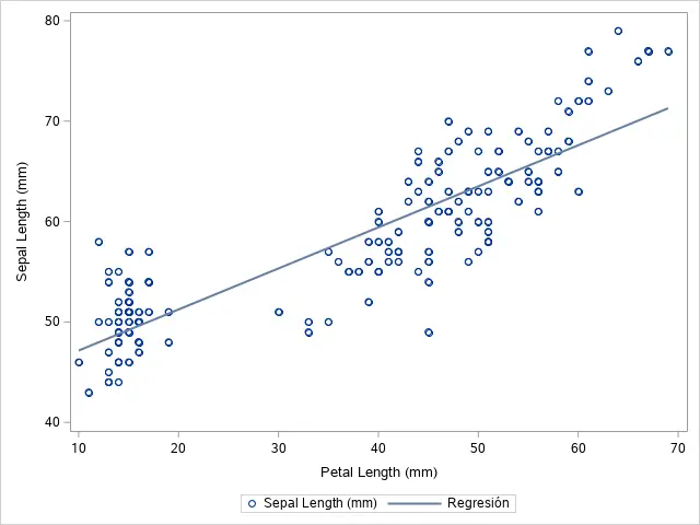
The following example shows how to add a regression line to a basic scatter plot.
proc sgplot data=sashelp.iris;
    scatter x = petallength  y = sepallength;
    reg x = petallength  y = sepallength;
run;
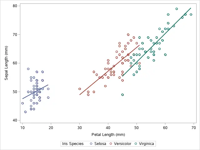
You can also add regression lines to a grouped scatter plot. Similar to the SCATTER statement, you need to add the group=-option to the REG statement to create a regression line for each group.
The SAS code below contains an example.
proc sgplot data=sashelp.iris;
    scatter x = petallength  y = sepallength / group=species;
    reg x = petallength  y = sepallength / group=species;
run;
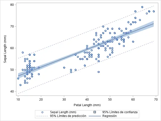
Additionally, you can add extra arguments to the REG statement to enhance the regression lines. The 2 most used optional arguments are CLM and CLI. Both add confidence bands to your plot, but are slightly different:
- CLM: The CLM option adds confidence limits for the mean predicted values.
- CLI: The CLI option adds confidence limits for the individual predicted values.
For example.
proc sgplot data=sashelp.iris;
    scatter x = petallength  y = sepallength;
    reg x = petallength  y = sepallength / clm cli;
run;
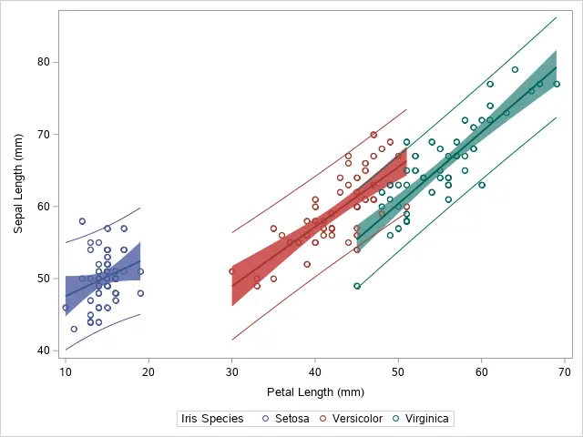
Likewise, you can also add confidence bands of regression lines to a grouped scatter plot.
proc sgplot data=sashelp.iris;
    scatter x = petallength  y = sepallength / group=species;
    reg x = petallength  y = sepallength / group=species clm cli;
run;
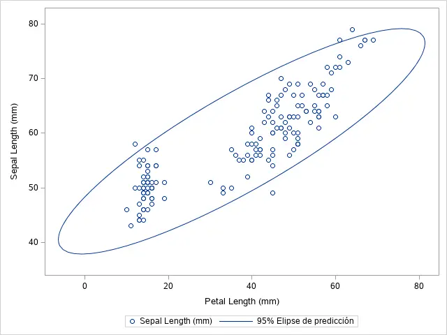
How to Add a Confidence Ellipse to a Scatter Plot
Besides regression lines, you can also use SAS to add a confidence ellipse to a scatter plot.
You can add a confidence ellipse to a scatter plot with the ELLIPSE statement. The ELLIPSE statement starts with the ellipse keyword followed by the x- and y-variables. In general, the x- and y-variable of the confidence ellipse are the same as the x- and y-variable of the SCATTER statement.
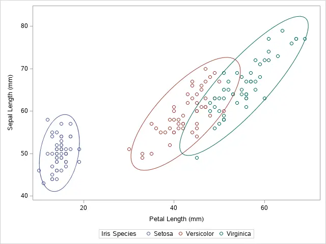
You can create both a confidence ellipse for a basic scatter plot, as well as for a grouped scatter plot. Below we show 2 coding examples.
proc sgplot data=sashelp.iris;
    scatter x = petallength  y = sepallength;
    ellipse x = petallength  y = sepallength;
run;
proc sgplot data=sashelp.iris;
    scatter x = petallength  y = sepallength / group=species;
    ellipse x = petallength  y = sepallength / group=species;
run;
How to Change the Titles of a Scatter Plot
By default, a scatter plot in SAS doesn’t have a title. Moreover, the labels (or titles) of the x-axis and y-axis are, by default, the labels of the corresponding variables. In this section, we explain how to change the titles of a scatter plot.
You can change the titles and labels of a scatter plot with the TITLE statement, the XAXIS statement, and the YAXIS statement. You use the TITLE statement for the overall title, while the XAXIS and YAXIS statements allow you to change the labels of the x-axis and the y-axis.
To change the title of a scatter plot you need a TITLE statement. This statement starts with the title keyword and the desired title between (double) quotes.
To modify the title (or labels) of the axes you need the XAXIS or YAXIS statement. After the keyword, you use the label=-option to define the title of the axis. You must write the title between (double) quotes.
Alternatively, you could change the label of the variable.
This is a coding example of how to modify the title and the labels of the axes:
proc sgplot data=sashelp.iris;
    scatter x = petallength  y = sepallength;
    title 'Scatter Plot of Patel Length and Sapel Length';
    xaxis label = 'Patel Length of Iris Flowers';
    yaxis label = 'Sepal Length of Iris Flowers';
run;
Do you know: How to Change the Size, Font, and Color of a Title in SAS?
How to Create a Matrix of Scatter Plots in SAS
Lastly, we discuss how to create a matrix of scatter plots in SAS.
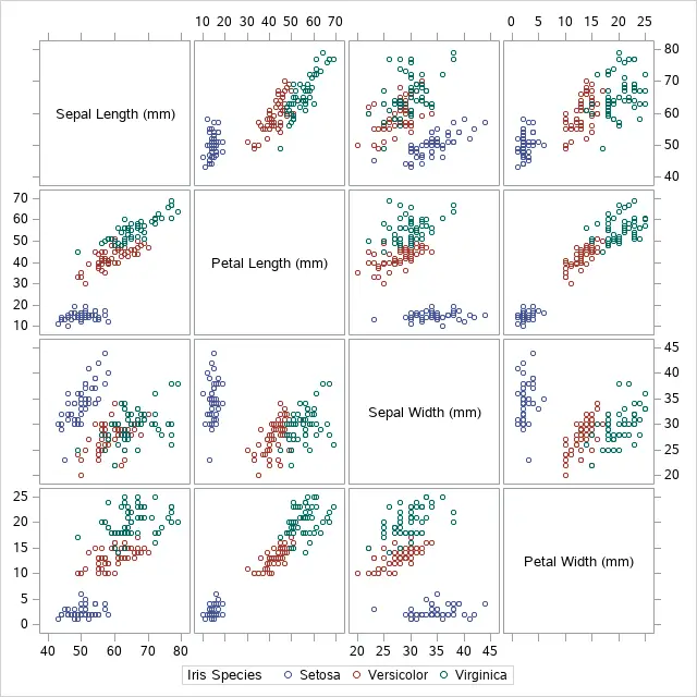
A scatter plot matrix is a matrix that contains one scatter plot for every possible combination of two variables. This type of scatter plot is useful to compare quickly the distribution of your data among all (selected) variables.
You create a scatter plot matrix in SAS with the SGSCATTER procedure. First, you specify the input dataset with the data=-option. Then you use the MATRIX statement to define the variables you want to include in the matrix. Additionally, you can add the group=-option to group the data.
The example below shows how to create a scatter plot matrix of all 4 variables in the Iris dataset grouped by the species variable.
proc sgscatter data=sashelp.iris;
    matrix sepallength petallength sepalwidth petalwidth / group=species;
run;
You can enhance the scatter plot matrix by adding extra statements to your code. For example, the REG statement for regression lines.

4 thoughts on “How to Create a Scatter Plot in SAS [Examples]”
Comments are closed.